1. Introduction
Those who are not familiar with the manufacturing industry may find the phrase Industry 4.0 difficult; however, it actually refers to the 4th industrial revolution, a phrase in the evolution of mankind’s manufacturing processes. There have been 3 Industrial Revolutions in history, the first of which occurred in Britain during the 18th century, with mechanization. The Second Industrial Revolution occurred in the early 20th century, and it was marked by improved industrial methods and assembly lines. The deployment of digital technology ushered in the Third Industrial Revolution in the 1960s. As computers became more powerful and the internet became more interconnected than ever before, Industry 4.0 began to take shape.
2. Advantages of using the Industry 4.0 model
- It makes you more competitive, particularly against disruptors such as Amazon.
- It increases your appeal to the younger workforce.
- It strengthens and encourages collaboration within your team.
- It helps you to handle possible concerns before they become major issues.
- It enables you to cut costs, increase earnings, and fuel growth.
3. What does CNCTrain offer in Industry 4.0?

- Automation
- Simulation
- Internet of Things (IOT)
- Visualization
- Robotics
- Additive Manufacturing
4. Software offered by CNCTrain for above six pillars
4.1. Node-RED for Automation and Internet of Things (IOT)
4.1.1. About Node-RED Software
Node-RED is a programming tool originally developed by IBM’s Emerging Technology Services team and now it is a part of OpenJS Foundation for connecting hardware devices, APIs, and online services in very interesting ways. It also provides a browser-based editor that will help you to wire together flows very easily.
4.1.2. System Requirements
Supported version of Node.js
No other requirements
4.1.3. Features of Node-RED Software
It provides browser-based flow editor that makes it easier to wire.
You can create JavaScript functions.
It is built on Node.js.
It can run on low cost hardware such as Raspberry Pi as well as in the cloud.
Flows created are stored using JSON which can be easily imported or exported for sharing purpose.
4.2. Ansys for Simulation
4.2.1. About Ansys Software
If you've ever watched a rocket launch, flown in an airplane, driven a car, used a computer, touched a mobile device, crossed a bridge, or put on wearable electronics, chances are you've used a product that utilizes Ansys software. Ansys is the global leader in engineering simulation, enabling next-generation developments such as self-driving cars, electric aircraft, and smart cities. The Ansys community assists people in overcoming the most difficult design issues and producing products that are only limited by their creativity by providing the greatest and most comprehensive portfolio of engineering simulation tools.
4.2.2. System Requirements for Ansys Software
64-bit Intel or AMD system and running Windows 10
8 GB Ram
A dedicated graphics card with the most recent drivers, at least 1GB of video RAM, and the ability to run DirectX 11 or higher. The Analyze stage in Discovery does not support or recommend the use of integrated graphics, such as Intel HD/IRIS.
3 button mouse
4.2.3. Features of Ansys
It can import all kinds of CAD geometries like 2D and 3D from different CAD softwares
It can perform advanced engineering simulations accurately
It is also capable of optimizing various features like geometrical design, boundary condition, etc
ACT is their own customized tool which uses python as a background scripting language
It has ability to perform analysis and integrate various physics
Can stimulate interaction between physics like dynamic, static and fluid
4.2.4. Applications
Antenna design and placement
Battery cell and electrode
Battery simulation
Autonomous software development
Flight control
3D design
Multiphysics
Electronics
4.2.5. Why Ansys Software is Important?
4.2.5. Why Ansys Software is Important?
Multinational companies like Honeywell, Raytheon, RTX, SpaceX, etc use Ansys Workbench. You can get a very accurate and reliable simulation in its Computational Fluid Dynamic analysis. Comparing it with other CAD software will also result in the best simulation and analysis software. Some fields of application of ANSYS which are open for Mechanical engineer are listed below:
Composites
Customization
Dynamics
Hydrodynamics
Multiphysics
Nonlinear Applications
Optimization
4.3. SciDAVis for Visualization
4.3.1. About SciDAVis Software
SciDAVis is a free interactive application for data analysis and plotting of publication-quality plots. It combines a short learning curve and it has a user-friendly graphical user interface with powerful features like scriptability and extensibility. SciDAVis runs on GNU/Linux, Windows, and MacOS X; it may also run on other platforms such as *BSD, though this has not been tested. In terms of its range of use, SciDAVis is comparable to both paid Windows programs like Origin and Sigma Plot as well as open-source programs like Qti plot, Lab plot, and Gnu plot. In contrast to the examples above, SciDAVis places a strong emphasis on creating a welcoming and open atmosphere (in the project as well as the software) for both novice and seasoned users. This specifically means that we'll work to offer excellent documentation at all levels, from user guides to tutorials and documentation of the internal APIs and beyond.
4.3.2. System Requirements for SciDAVis software
You need to install Python 2.5 to run this software.
No other system requirements needed.
4.3.3. Key Features of SciDAVis software
Here is a quick review of what SciDAVis is capable of. If you're still not sure if it will work for you, you can just download SciDAVis and try it out for yourself!
You can gather tables (2D data), matrices (3D data), graphs (2D or 3D plots) and notes (text notes or scripts) in a project which can be organized using folders.
You can directly enter data for tables or matrices or it can also be imported from ASCII files.
Standard and special functions can be used to calculate the values of the cells in tables (and much more if you have Python installed) and you can assign individual formulas to each table cell.
For tables and matrices you can perform Multi-level undo/redo.
There are numerous built-in analysis operations available including column/row statistics, (de)convolution, Fast Fourier Transform (FFT) and FFT-based filters.
You can get extensive support for multi-peak fitting, fitting linear and nonlinear functions to the data.
You can export 2D plots such as symbols/lines, bars and pie charts in various different formats like JPG, PNG, EPS, PDF, SVG and more.
You can export Interactive 3D plots to a variety of formats including EPS and PDF.
You can even access additional project objects with Python installed, for example, to quickly write an import filter for a custom data format.
4.3.4. Used cases of SciDAVis software
4.3.4.1. Drawing Plots:
→ 2D X-Y plot
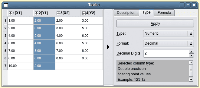
Create a new table and enter its dimensions to be 4 columns and 7 rows. Select the third column and Set Column as command to set it as X from the Table menu. You can then enter the values of two series i.e (X1,Y1) and (X2,Y2) as shown in figure 2.
Use the Plot menu to create the plot by selecting the two Y columns (select Y1, Y2 with CTRL key) and use the Plot command to create a straightforward plot with two axes. Then choose the data series for which you want to modify the axes in the left window, then click the axis tag and choose the axes you want to use. You will see that the plot is now changed, but the new axes are not displayed so choose the new axes using the Axes command, then click on the show checkbox. You can then customize your plot according to your need to obtain the result presented in fig 3.
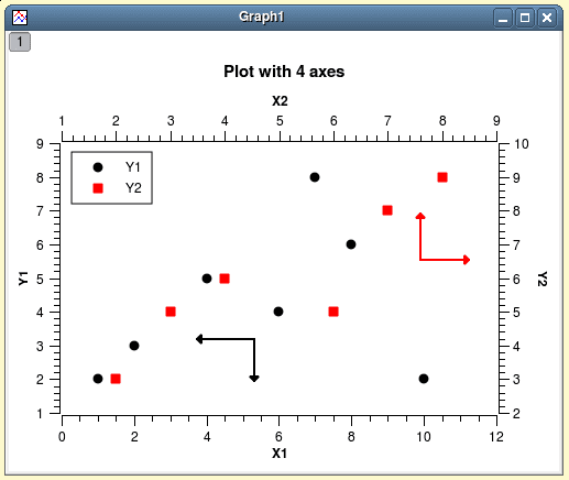
With the help of the Format menu's commands, you can modify/change your plot and you can edit the symbols by double clicking on the data points to access the Plot command dialogue. Once the Axes command dialogue has been opened, you can change the scales, the typefaces used for the axes labels, etc. by double-clicking on the axes. Grid command allows you to add grid lines to the X or Y axes. The text and presentation of any text item (X title, Y title, plot title) can be changed by double clicking on that item.
→ 2d Plot from function
Use the New → New Function Plot command from the File menu or press CTRL+F to simply plot a function. You can also use icon available in file toolbar. You can then enter the expression of your mathematical function, the X range used for the plot, and the number of points used in this X range.
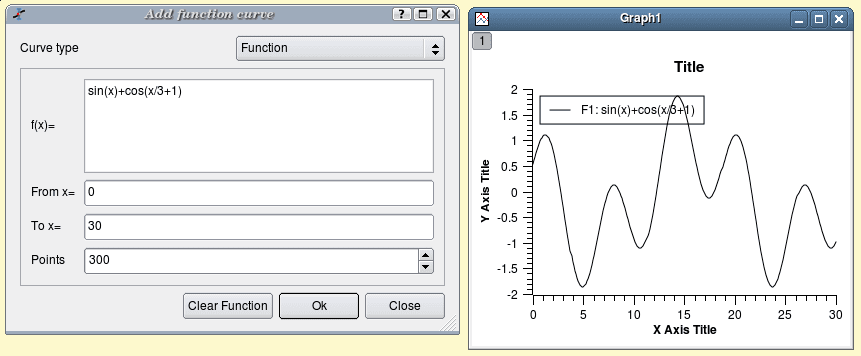
The generic plot which is created by this command can be customized as explained in the earlier section.
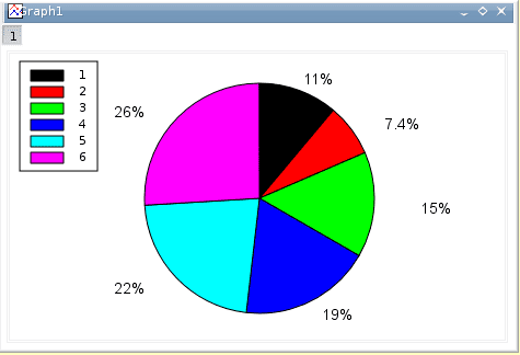
→ 2D Pie Plot
A table with two columns can be used to create a pie plot; the first column will be treated as text, and the second as numbers. By default, there will be one label with the percentages calculated from the Y values in each sector of the plot. These labels are flexible, just like any other text label.
→ Statistical Plots - Box Plot
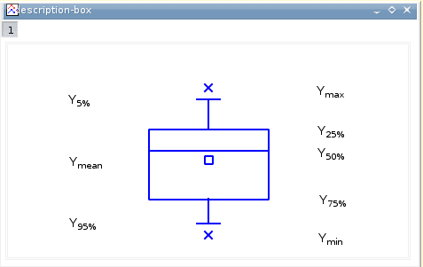
The important characteristic of Box plot is data distribution which is used to display various statistical values. For example, Let us assume that we have a table with a column that has 12 values. You will get a graph that is similar to the one shown in the figure 6 if you choose this column and use the Statistical graphs → Box Plot command to create a box plot. By default, the values which are computed from your data are as follows:
- Ymax is the maximum value of Y.
Y5% is the value of Y compared to the top 5% of the distribution of numbers.
Y25% is the value of Y compared to the top 25% of the distribution of numbers.
Y50% is the value of Y compared to the top 50% of the distribution of numbers (also known as the median value).
Ymean is the average value of Y.
Y75% is the value of Y compared to the top 75% of the distribution of numbers.
Y95% is the value of Y compared to the top 95% of the distribution of numbers.
Ymin is the minimum value of Y.
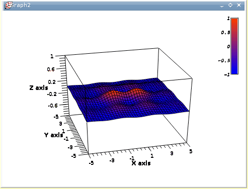
→ 3D Plots from a function
This is the most simple method for obtaining a 3D plot. Just select the File menu→ New → New 3D Surface Plot command or by pressing CTRL+ALT+Z. The following dialogue box will appear:
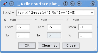
You can then write the function z = f(x,y) and specify the X, Y, and Z ranges. After that, SciDAVis will create a standard 3D plot:
4.3.4.2. Analysis of Data and Curves using Fast Fourier Transform
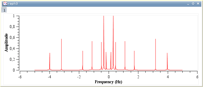
When a table or plot is selected, the FFT command of the Analysis-tables menu or the Analysis-plots menu will take you to this function. The Fourier transform breaks down a signal into its component parts by assuming that the signal x(t) can be described as a sum:
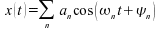
where, 𝛚n is the frequency, an is the amplitude of each frequency and n is the phase corresponding frequency. SciDAVis will calculate these parameters and create a new plot of amplitude versus frequency. Then you can use FFT to extract the characteristic frequencies from a curve. Let's assume you have the signal depicted in the following figure 9. To open the FFT dialogue box, select the FFT command from the Analysis-plots menu.
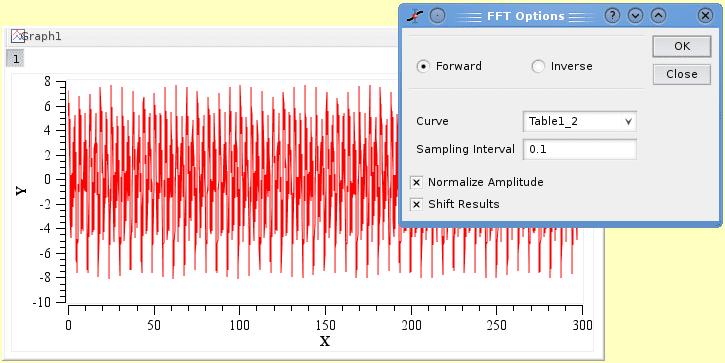
If you select the Normalize Amplitude check box the amplitude curve will be normalized to 1. If the Shift Results check box is selected, the frequencies are shifted to produce a centered X-scale. The Sampling Interval is set to the interval between X-values by default. Giving a lower value makes no sense, but you can raise it to sample fewer values. SciDAVis will generate a new plot window with the FFT amplitude curve and a new table with the real, imaginary, amplitude, and angle of the FFT. The amplitude curve in this example has been normalized, and the frequencies have been moved to obtain a centered X-scale.
In the case of a table, you must choose the sampling column (X-values) and one or two columns (for complex numbers) for Y-values.

4.4. M-Robot for Robotics
4.4.1. About M-Robot Software
It is an introductory 3D software which is used for programming and simulation purposes. This software also allows the trainees to learn some interesting and cool robot techniques in a safe environment. There are ready-made applications available that will train you in robot activities such as movement, programming and code production. You can also create new objects and import them into the software. This software also allows you to include graphics.
4.4.2. Key Features of M-Robot
It is easy to use.
You can do Axis and Cartesian programming.
Provided with teach pendant.
Teach command programming.
Easy to travel through software and machine controls are also simple.
4.4.3. What you can do in the software?
4.4.3.1. Execution:
In this tab you can write code or simply import the code file. Click on the E symbol available at the top right corner to open the editor. In editor you can simply type the code or else import the file as shown in figure 12 and 13:
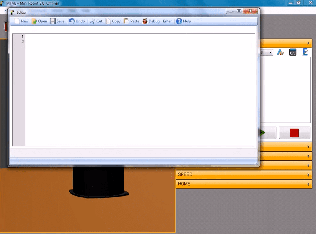
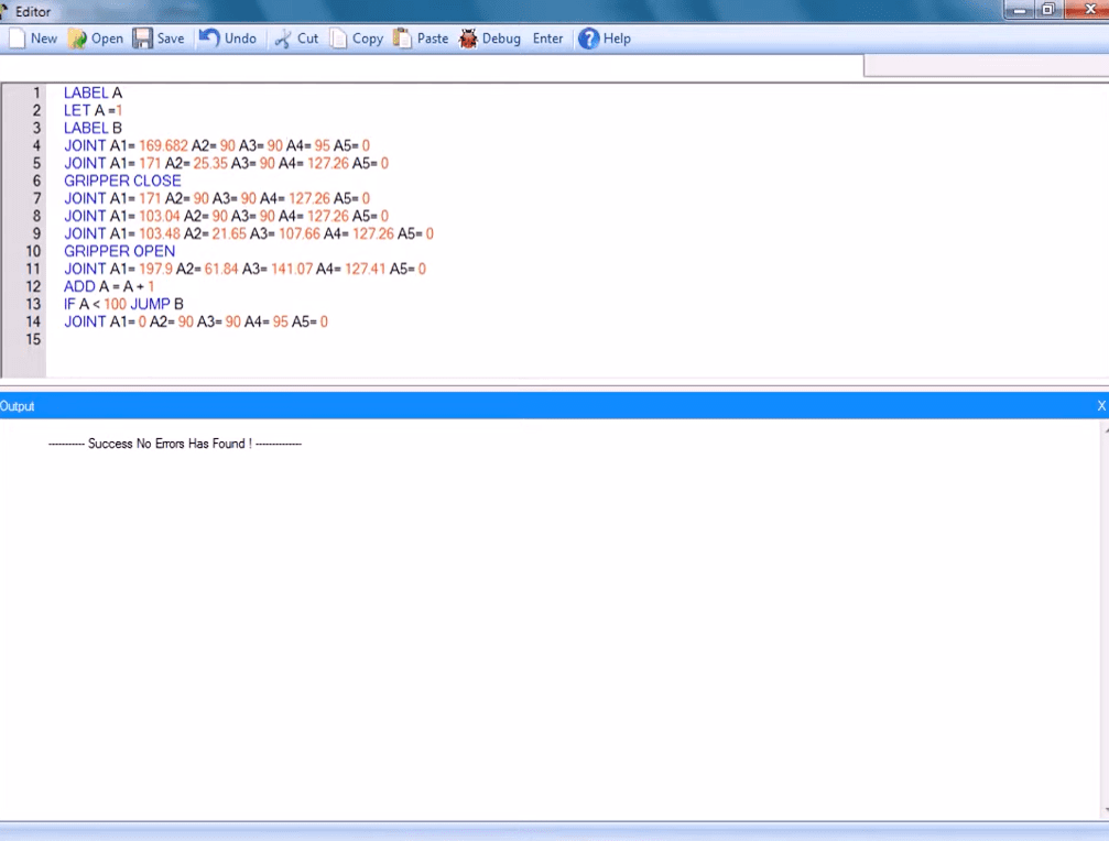
Now click on Enter button to import the code to the execution tab and then click on the Run button.
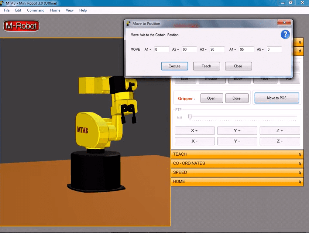
4.4.3.2. JOG:
There are different features available under this category they are as follows:
You can use Base+ and Base- to change its base position.
You can use Shoulder+ and Shoulder- to change shoulder position.
You can use Elbow+ and Elbow- to change Elbow position.
You can use Pitch+ and Pitch- to change Pitch of the robot.
You can use Roll+ and Roll- to roll the gripper in desired position.
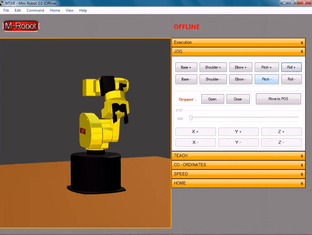
You can also use the Move to POS button to move the axis to cartesian position. You just need to input the required values as shown in fig 15 and just click on the Execute button.
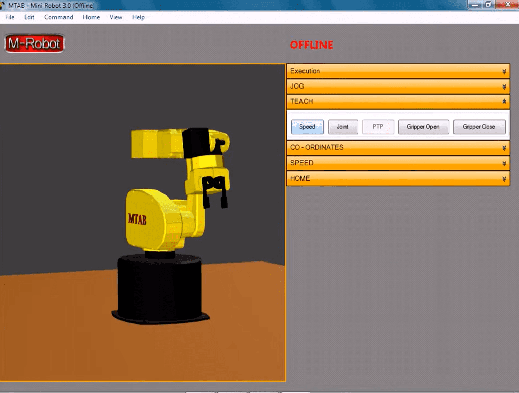
4.4.3.3. Teach:
It provides with different features like speed, Joint, PTP, Gripper Open and Gripper Close as shown in the figure 16:
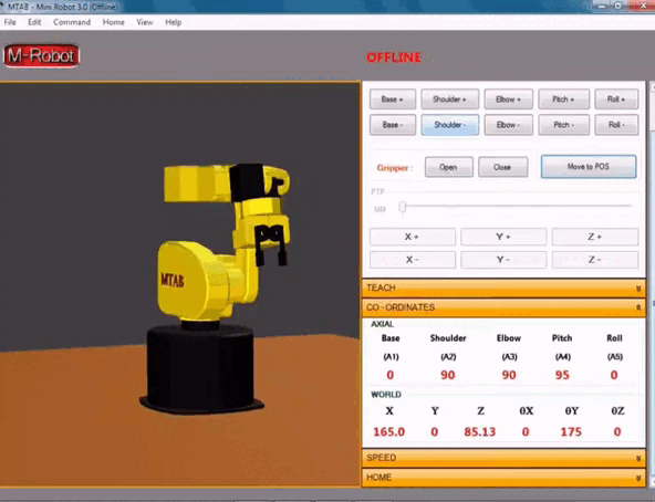
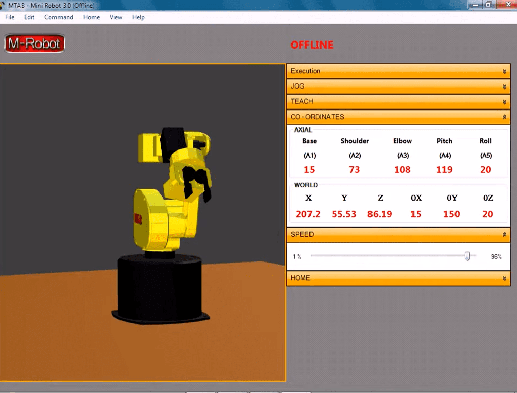
4.4.3.4. Co - Ordinates:
You can verify how your coordinates are changing by watching the animation below:
4.4.3.5. Speed:
You can adjust your robot's moving speed. It depends on how fast or slow you need it to perform.
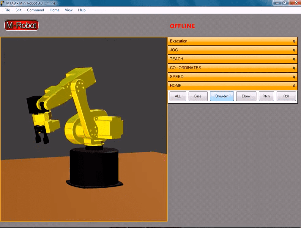
4.4.3.6. Home:
Under the home tab different functions are available which includes All, Base, Shoulder, Elbow, Pitch and Roll. You can change the coordinates by simply clicking it.
4.5. Ultimaker Cura for Additive Manufacturing
4.5.1. About Ultimaker Cura Software
For 3D printers, Cura is an open source slicing program. It was developed by David Braam who eventually became a software maintenance employee of Ultimaker. Cura is distributed under the LGPLv3 license. Cura was initially released under the open source Affero General Public License version 3, but the license was changed to LGPLv3 on September 28, 2017. This modification enabled greater integration with third-party CAD applications. It has over one million users worldwide and processes 1.4 million print jobs per week. It is the preferred 3D printing software for Ultimaker 3D printers, but it is also compatible with other printers.
4.5.2. System requirements for Ultimaker Cura
4.5.2.1. Minimum System Requirements
Your graphics card should be compatible with OpenGL 2. For 3D layer view OpenGL 4.1 is preferred.
Your display resolution should be 1024 x 768.
Processor should be Intel core 2 or AMD Athlon 64 or above.
550 MB space available on hard disk drive.
4 GB Ram memory.
4.5.2.2. Recommended System Requirements
OpenGL 4.1 compatible graphics card for 3D layer view.
1920 x 1080 pixels should be your display resolution.
Processor should be Intel core i3 or AMD Athlon 64 or above.
600 MB space available on hard disk drive.
8 GB Ram memory.
4.5.3. Technical Specifications
The way Ultimaker Cura operates is by creating a printer-specific g-code and by slicing the user's model file into layers. After it is complete, the g-code may be transferred to the printer for manufacturing of physical objects.
It can work with files in the most popular 3D formats, including STL, OBJ, X3D, and 3MF, as well as picture file formats, including BMP, GIF, JPG, and PNG. It is also compatible with the majority of desktop 3D printers.
4.5.4. Key Features
- Slicing Feature:
Recommended profiles are tested for thousands of hours which ensures reliable results.
For finer control ‘Custom Mode’ offers over 400 settings.
Updates are made at regular intervals to improve features and printing experience of users.
You will be able to continuously integrate with all Ultimaker products.
You will be able to integrate CAD plug-ins with SolidWorks, Siemens NX, Autodesk Inventor and more.
Supported file formats are STL, OBJ, X3D, 3MF, BMP, GIF, JPG, PNG.
You can prepare your 3D model for printing in minutes with recommended settings.
You can just select the speed and quality settings, and you can start printing.
It is open source and costs nothing to use.
For your application, you can download material profiles from leading brands.
You can avoid manual setup when using 3rd party materials.
Download helpful plugins to customize your print preparation experience, star-rated by community.
Ultimaker Cura Enterprise can be deployed, configured, and managed with cross-platform systems distribution.
Ultimaker Cura Enterprise receives two updates per year. They are thoroughly tested by the community and it is guaranteed that it has a more stable desktop application.
Each instance of Ultimaker Cura Enterprise is independently scanned, tested, and analyzed for virus and threats.
Slicing features are listed below:
At one click intent profiles print specific applications
2. Integrated Workflow:
If you own a 3D printer, it all comes down to software. Workflow features listed below:
3. Easy to use:
Manufacturing should not be made complicated so the software is designed for absolute beginners as well as experienced 3D developers. Some of the features listed below:
4. Ultimaker Marketplace:
Openness and cooperation are in our DNA. Some of the features include:
5. Ultimaker Cura Enterprise:
Ultimaker Cura Enterprise delivers stability and security with business-friendly features. Some of the features include:
5. Conclusions
As we have already discussed about the importance of IOT it is necessary to upskill yourself in respective domains. In this article, we have discussed many important tools/software which can be used. Node-RED can be used for Automation and IOT purposes. We can make use of SciDAVis for Visualization purposes. We can use Fast Fourier Transform to visualize the data in SciDAVis. M-Robot has been used for Robotics in which you can animate the actual robot and verify how coordinates are changing. Ultimaker Cura is used for Additive Manufacturing where you can create 3D printings. Many industries have already been using Ultimaker Cura. For eg: Idea reality created 3D prototype, Ford used 3D printed Jigs and tools in there manufacturing line and ZEISS printed Adapter plate.
FAQs
Q1) What is Industry 4.0?
→ Industry 4.0 is the next industrial revolution, characterized by the connectivity of industrial equipment and continuous data flow to access and evaluate consolidated information.
Q2) What are the benefits of Industry 4.0 for organizations?
→ Asset efficiency & productivity, better quality product with less number of defects, cost reduction, greater sustainability, safer and more flexible & agile.
Q3) How can I visualize data from a text file in SciDAVis?
→ Select the Import ASCII -> Single File command from the File menu. If the file does not import correctly, use the Set Import Options command from the File menu to modify the column separator. TAB is the default column separator.
Q4) Why should I prefer M-Robot over other applications?
→ This software allows trainees to learn robot teaching techniques in a safe environment and also ready-made applications are available to train the user in the operations of the robot such as movement, programming and code generation.
Q5) What is flow-based programming in Node-RED?
→ It is a way of describing an application’s behavior as a network of black boxes or nodes.
Q6) On what operating systems is Ultimaker Cura available?
→ It is compatible with following operating systems:
Windows 10 or higher, 64 bit
Mac OSX 10.15 or higher, 64 bit
Linux, 64 bit
Incompatible operating system:
Chrome OS
Virtual Desktop applications / operating systems
Windows 7 or older
Mac OS 10.14 and older
